Setup ESP8266

What: Setup a ESP8266 by installing fresh NodeMCU firmware
Why: Update firmware and get cheap Esp’s which come without NodeMCU up and running
How: Use NodeMCU-PyFlasher and Docker to flash Esp, build firmware and put it on the Esp

Install docker

If you have no docker installed already, install it. You can use the script below (execute as root, see here).

apt-get install -y --no-install-recommends apt-transport-https ca-certificates curl software-properties-common
curl -fsSL https://apt.dockerproject.org/gpg | sudo apt-key add -
add-apt-repository "deb https://apt.dockerproject.org/repo/ debian-$(lsb_release -cs) main"
apt-get update
apt-get -y install docker-engine

Build the firmware

Clone the NodeMCU firmware from github (see here):

git clone https://github.com/nodemcu/nodemcu-firmware.git

Edit the file app/include/user_modules.h. Here you can enable further modules, for example http-module for http requests. For enabling a module, remove the comment markers at the beginning of the line.

Edit the file app/include/user_config.h and enable ssl. As above, this is done by removing the comment markers at the beginning of the line.

Change to the directory and start docker for NodeMCU build (see here):

sudo docker run --rm -ti -v `pwd`:/opt/nodemcu-firmware marcelstoer/nodemcu-build

You should now have two bin-files (for example nodemcu_float_master_20170228-2105.bin) in the bin-folder: One for the integer version and one for the float version.

Flash the firmware to the ESP

Connect the ESP to the USB port of your computer and start the NodeMCU-PyFlasher. Select the correct serial port (you can find it in the device manager, com ports; USB-SERIAL). Select the image file created above. Select the erase flash option and click on Flash NodeMCU.

It should take some time (approx. 1 min). You should see the message „– verify OK (digest matched)“. Now, you have a freshly installed NodeMCU on the Esp. Enjoy!

Setup Raspberry Pi with WLAN and ssh from start

What: Setup Wlan on a fresh raspberry without ethernet cable
Why: Fast and headless setup while still sitting on the couch
How: Use the latest raspbian image, provide wpa_supplicant.conf and ssh file

Download raspbian image

Download the zipped image file from here. I took the raspbian jessie lite.

Unpack it.

Put the image on a SD card

Use a suitable SD card (mine is 8GB) and format it. You can use SDFormatter on Windows for that.

Afterwards, copy the image file to the card. You can use Win32DiskImager for that.

Setup Wlan and ssh

Go to the SD card drive. There should be a file called cmdline.txt.

Create a new file called wpa_supplicant.conf in the same directory like the cmdline.txt and put the following in (Update: The lines changed between Raspbian Jessie and Stretch, see here):

ctrl_interface=/var/run/wpa_supplicant
network={
    ssid="your-network-ssid-name"
    psk="your-network-password"
}

This step is taken from here.

Since december 2016, ssh is by default disabled in raspbian. To enable it, create a new and empty file called ssh in the same directory like the cmdline.txt. See documentation.

Start the raspberry

Put the SD card into the raspberry and start it. The raspberry should now be visible in your network and you should be able to establish a ssh connection via Wlan. For the first raspberry start it may take some time (3 min. in my case) but for further restarts the raspberry was available via ssh within seconds.

Vim forever

What: Installing Vim one every machine you work with
Why: Avoid complicated setup of the favourite IDE each time on a new (virtual) machine
How: Using Ansible to install and pimp Vim

Vim is a great IDE, but with some plugins it is even better. I regularly use and want to have the following plugins available:

Install vim on multiple machines is quite simple with Ansible. See my other blog entry for installing ansible and a first toy example of ansible in action.

Install and pimp Vim

Install Ansible on your system and clone my blog repository. It contains the playbook (vim.yml) and a helper file (installVim.sh).

Note: If you use the playbook to install and pimp Vim on the same machine like ansible is running: Clone to a different location than /tmp/blog. Use /tmp/bloginstall for example.

1
git clone https://github.com/frankdressel/blog.git /tmp/bloginstall

In the blog/ansible directory you will find the playbook file vim.yml. By default, it is configured to install Vim on a test remote machine (if you are using Vagrant, you can find the Vagrantfile here). If you don’t want this, change the following line and replace ansibletest with your remote machines name.

  hosts: ansibletest
  hosts: your_machine_name

Afterwards, run the playbook with the following command (password based authentication is used here with the option –ask-pass, see here):

1
2
cd /tmp/bloginstall/ansible
ansible-playbook vim.yml -u  --ask-pass --ask-become-pass

If you want to run it on your local machine use the following instead:

ansible-playbook -i "localhost," -c local vim.yml

Ansible will produce some output which should end with something like:

1
2
PLAY RECAP *********************************************************************
10.0.2.2                   : ok=17   changed=0    unreachable=0    failed=0

If you are a linux user: Done! If you are using Windows and putty, there is one last step to be done to have a nice user experience with power line: Change the font used on your vim terminal. See this blog for the setup. It is done in less than 5 minutes. By default, the Vim instance presented here is using the DejaVu Sans Mono for Powerline font as described in the tutorial.

Machines should work: Using Ansible for IT VM provisioning

What: System provisioning
Why: Faster development startup
How: Using Ansible modules for provisioning via ssh

During the what the data hackathon, a friend of mine and I used Vagrant for setting up the same system for both of us. It was a perfect starting point. Nevertheless, during hacking we installed this package, tried out that package, .. After a short while, the two systems were not equal anymore. This is a first approach to use Ansible to keep two machines in sync during development.

Ansible works by using a central machine (control machine) to provision other machines (remote machines) via ssh. In this tutorial the control machine is assummed to be a linux machine with Python < 3 installed and the remote machine is a Vagrant VM running debian (see here for the Vagrantfile).

Additional resources

See also: this blog

Ansible Installation

In principal, it should be possible to install Ansible from source (github). Nevertheless, I already had Anaconda with Python 3 installed on the controll machine, which complicated things a little bit because Ansible works only wih Python < 3. After some trial and error, I installed Ansible using pip. You have to install the dependencies before:

1
2
sudo easy_install pip
sudo pip install paramiko PyYAML Jinja2 httplib2 six

If you get an error message about missing libffi, install python-cffi before.

Install Ansible via pip:

1
sudo pip install ansible

Setup Ansible

You have to setup Ansible by providing a so called Inventory file to specify, which machines should be provisioned.
Create a file called hosts and add a name in brackets as well as ip, port, … for all the machines you want to provision. If you use the Vagrantfile from here, the ip should be 10.0.2.2 (default gateway in Vagrant for public networks). In other cases or if no connection is established change the ip accordingly. You can find the ip by running the following command on the remote machine. Look for the address which is listed as default gateway ip.

1
/sbin/ifconfig

With the correct ip, create the inventory file:

1
2
3
4
cat &lt;&gt; /home/vagrant/ansible/hosts
[ansibletest]
10.0.2.2 ansible_port=2200 ansible_user=vagrant
EOF

Ping

Ansible uses key based authentification by default. I switched it off in my use case for simplicity and use password based authentication which is enabled by –ask-pass. Otherwise, the keys have to be set up. For password based authentication: You have to install sshpass.

Ansible comes with a predefined module for checkin availability of remote machines: ping. Use it with the -m option:

1
ansible ansibletest -i  -m ping --ask-pass

You will be asked for the password on the remote machine (it is vagrant) and after that the output should be equivalent to:

1
2
3
4
10.0.2.2 | SUCCESS =&gt; {
    "changed": false,
    "ping": "pong"
}

Installing Python3, pip and Pandas on the remote machine

Ansible works by executing so called playbooks for different scenarios.

Lets create a playbook, which uses apt to install Python 3 and pip on the remote machine and afterwards using pip to install python packages (Pandas in this case). Create a file called python-datascience.yml with the following content (or download it here):

1
2
3
4
5
6
7
8
9
10
11
12
13
14
15
16
17
18
19
---
- name: install python for data science
  hosts: ansibletest
  become: true

  tasks:
    - name: Get aptitude for upgrade
      apt: pkg=aptitude state=present

    - name: install base packages
      apt: pkg={{item}} state=present
      with_items:
        - python3
        - python3-pip

    - name: Install global python requirements
      pip: name={{item}} state=present executable=pip3
      with_items:
        - pandas

Run this playbook in a way similar to the ping above:

1
ansible-playbook python-datascience.yml --ask-pass

The output should be:

1
2
3
4
5
6
7
8
9
10
11
12
13
14
15
16
PLAY [install python for data science] *****************************************
 
TASK [setup] *******************************************************************
ok: [10.0.2.2]
 
TASK [Get aptitude for upgrade] ************************************************
ok: [10.0.2.2]
 
TASK [install base packages] ***************************************************
ok: [10.0.2.2] =&gt; (item=[u'python3', u'python3-pip'])
 
TASK [Install global python requirements] **************************************
ok: [10.0.2.2] =&gt; (item=pandas)
 
PLAY RECAP *********************************************************************
10.0.2.2                   : ok=4    changed=0    unreachable=0    failed=0

Login to the remote machine to check the result. You should have python3 and pandas now installed.

Let the sun shine

What: Getting power production data in a real life photovoltaic system
Why: Use real data in modelling; Use mqtt to get sensor data
How: Use mqtt, csvkit and R to get and clean the data, use command line pipeline for data processing

This is the second part of my what-the-data hackathon series. Please visit also part one.

During the hackathon, the data were provided in json format with a timestamp. We collected data for nearly two days without serious interruption. My team was looking at the power production of the photovoltaic system. We decided to gather all the data as-is and write it to disk (we were expecting <100Mb of data). We used a small python script to get the data via mqtt. After the two days we collected 2.7Mb of data for the power production (and a lot more for other sensor data), which is approx. 58.000 entries like:

b'{"value":-3724.951,"timestamp":1474813391427}'
b'{"value":-3746.143,"timestamp":1474813392417}'

You can download the file here.

We needed the data for simulation, where we simulated energy transport in the system for each second. Most of the data were already timed at seconds, but some data points were missing due to sensor failures. Nevertheless, for our simulation we needed also values for these timepoints. Luckily, the sun shine doesn’t change too fast and a simple smoothing was enough to interpolate missing values.

We wanted to process the data with R and maybe other tools. We decided to convert the data to csv and process this further. Main points of the decision were:

  • Ability to put csv easily under version control (text file)
  • Use the csv file in a ton of different tools

We used the following bash script to strip of characters and convert the single entries to a proper json array (assume, the raw data is in the file pv_wirk.raw and has the format described above):

1
2
3
sed "s/^b//g" pv_wirk.raw | sed "s/'//g" | \
sed "s/$/,/g" | sed '$s/},/}/g' | \
sed 's/value":-/value":/g' | sed "1 i \[" | sed -e "\$a]"

It does the following:

  1. Strips of the first character (b)
  2. Strips of the dash characters
  3. Adds a comma at the end of the line
  4. Removes the comma from the last line (althouh it is valid json, csvkit is a little bit picky about this)
  5. Inverts the data. This was needed because the produced power was send with a neative sign.
  6. Add a square bracket at the first line to begin the json array
  7. Add a square bracket at the last line to end the json array

The output of the above command is piped into csvkit and converted from json to csv:

1
... | csvkit -f json

The data is now in the form:

value,timestamp
4379.872,1474707052767
4388.521,1474707053773
4393.466,1474707054770

With the data in a nice csv format, we used R to plot the data and interpolate it simply by using loess smoothing. Where data were missing, we imputed it with predicted values from the loess-fit. You can find the R script here.

The resulting image is shown below. The power still shows the natural fluctuations but also contains data for each second.
analysed

What the data hackathon 2016: Agents on the run

The What the data hackathon is over! It was an incredible weekend in Hamburg with a lot of fun, nerds and crazy ideas (and some barbeque as well). A friend of mine and I were participating as team coding agents and we were one of the prize winning teams!

logo

The hackathon was held in a smart house of the Energie-Campus, Hamburg full of sensors. The sensors included heating, photovoltaic, hydrolysis and methane production for power2gas conversions, a lot of heat sensors, power consumption/production sensors on many systems, RFID tags and readers, cameras, lights, … All the systems were nicely available through MQTT protocoll and although the WiFi was off for some time and not all privileges to read/write data were granted from the beginning on, the organizers did a really great job! Thanks so much! During the hackathon we learned a lot about MQTT, renewable energy, smart houses, IoT, sensors and man-machine interactions. It is definitely worth to visit the hackathon next year again. And to show some numbers: According to the organizers 40 million data sets were transfered during the weekend between the hackathon participants and the sensor system.

This is the first part of articles about the hackathon. For further reading please see part two.

Following are some of my personal highlights of the event:

  • A team using Alexa, Mobile or a Smartwatch as input device for querying machine state. If a RFID tagged user was close to a machine Alexa was answering a simple command with a detailed explanation of the machines state like: CO2, O2 or Methane concentration, temperature, …

    alexa

  • A team using a laser scanner on the fridge to trigger a camera, which made a photo of the fridge opening persons T-shirt. The image was analysed with respect of T-shirt color and bound to the persons rfid-id. Next time this person was close to any of the RFID readers its color changed according to the T-shirt color. All the data were visualized with a small app. A nice and simple way to play Capture the flag.

    capture-the-flag

  • A team proposing blockchain technology to organize energy distribution based on the demand of an individual agent. Maybe, things like that can be done with smart contracts? The different parts in the system are independent agents, the hydrolysis machine was used as an example.

    blockchain

  • A team using a smartwatch as input device to control the movement of a roboter arm. The movement included up/down, left/right and stick/release items.

    robot

It was very interesting to see location based activation of services in different applications (capture the flag and alexa). For sure, this is a quite powerful concept also for serious applications. Also, the use of Raspberries in a lot of projects was very interesting. As an additional plus: Discussions with a lot of people about sensors, chips and how to use it for hobby projects.

Our own project was about simulating the energy distribution from the photovoltaic on the roof down to the different stages of hydrolysis, methan production to charging electrical bicycles and electrical cars. There was some time left at the end. We did a good investment by using this time to tought the RFID sensors to blink in Morse code during our final presentation.

morse

Some parts of our project will be highlighted here in future articles. Stay tuned!

Drake, drip & Data science

What: Analysing data with a data workflow, fast Java startup & csv Magic
Why: Building data analysis pipelines for (small) problems, where intermediate steps are automatically documented
How: Use Drake for (data) workflow management, Drip for fast JVM startup and csvkit for csv magic.

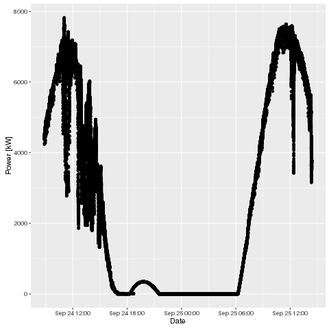
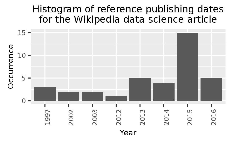
In this post, I will show you how to build a small data analysis pipeline for analysing the references of a wikipedia article (about data science). The result is the following simple image, all steps are automated and intermediate results are documented automatically.

result.plot

In the end, you should have four artifacts documenting your work:

  • Drakefile: The workflow file, with which you ca regenerate all other artifacts. Plain text, thus can be easily used with version control systems.
  • data.collect: The html content of the wikipedia article as the source of the analysis
  • data.extract: The publishing years of the references with number of occurrence
  • result.plot.png: A png of the publishing year histogram

Agenda

  1. Install the requirements
  2. Build the pipeline
  3. Run the pipeline

Install the requirements

You need the following tools:

  • Linux (Debian or Ubuntu, command line tools)
  • Python (for html processing and csv magic)
  • R (for plotting)
  • Java (for Drake)

You can install the dependencies easily with the script below. The following steps are tested within a Debian (Jessie) VM, 64bit. It should also work on Ubuntu. Maybe, other distros have to be adapted.

1
2
3
4
5
6
7
8
9
10
11
12
13
14
15
16
17
18
19
20
21
22
23
24
25
26
27
28
29
30
31
32
33
# Update
sudo apt-get update
 
# Install curl
sudo apt-get install -y curl
 
# Install R
sudo apt-get install -y r-base
sudo apt-get install -y r-cran-rcpp
sudo Rscript -e 'install.packages("ggplot2", repos="https://cran.uni-muenster.de/")'
 
# Install Java8
sudo sh -c 'echo deb http://ftp.de.debian.org/debian jessie-backports main >> /etc/apt/sources.list'
sudo apt-get update
sudo apt-get install -y openjdk-8-jdk
 
# Install Drip
mkdir ~/.lib
git clone https://github.com/flatland/drip.git ~/.lib/drip
cd ~/.lib/drip
make prefix=~/.bin install
 
# Download & Setup Drake
wget https://github.com/Factual/drake/releases/download/1.0.3/drake.jar -O ~/.lib/drake.jar
cat << 'EOF' > ~/.bin/drake
#!/bin/bash
drip -cp ~/.lib/drake.jar drake.core "$@"
EOF
chmod u+x ~/.bin/drake
echo export PATH=~/.bin:$PATH >> ~/.bashrc
 
# Install csvkit
pip install csvkit

Build the pipeline

Drake is controlled by a so called Drakefile. Let us define three steps for the data processing:

  1. Data collection (html from Wikipedia)
  2. Data extraction (Extracting the reference texts and years of the references)
  3. Plotting results (Plotting the results to png)

1. Data collection

The first step can be done with Linux internal tools. Thus, we can create the Drakefile with the first step already:

data.collect <- [-timecheck]
  curl -k https://de.wikipedia.org/wiki/Data_Science > $OUTPUT

Drake takes input (mostly) from files and sends the output of each step again to files. Thus, the result of each step in a workflow is automatically documented.

This first step will download the html for the data science article from the german wikipedia and stores the html in a file called data.collect (the [-timecheck] avoids running the step each time drake is started because of missing input from previous steps). You can already run this workflow with the drake command:

drake

This will generate a file called data.collect containing the html of the wikipedia page.

2. Data extraction

For data extraction from html, Python & BeautifulSoup is used. The extraction of the year from each reference can be done with linux internal tools (for example grep). Thus, the python program should read from stdin, get the reference text and outputs plain text to stdout. Create a file called extract.py with the following content:

1
2
3
4
5
6
7
8
9
10
11
12
#!/usr/bin/env python3
 
from bs4 import BeautifulSoup
import sys
 
input=sys.stdin.read()
soup=BeautifulSoup(input, 'html.parser')
 
entries=soup.find('ol', {'class': 'references'}).findAll('li')
 
for entry in entries:
    print(entry.getText())

Make the script file executable with:

chmod u+x ./extract.py

You can test the script with the following command (If you ran the workflow from step 1 before):

cat data.collect | ./extract.py

Now, let us extend the Drakefile to use the python script, search for years with a regex, create a histogram by counting the occurrences of the years, reorder the columns and add a header:

data.collect <- [-timecheck]
  curl -k https://de.wikipedia.org/wiki/Data_Science > $OUTPUT

data.extract <- data.collect
  cat $INPUT | ./extract.py | grep -o -P '\b\d{4}\b' | sort | uniq -c | sort -nr | \
    sed 's/^[ ]*//g' | csvcut -c2,1 -d " " | printf 'year, occ'"\n$(cat)" > $OUTPUT

If you run this workflow with:

drake

a new file called data.extract will be created which looks like the following:

year, occ
2015,15
2016,5
2013,5
2014,4
1997,3
2003,2
2002,2
2012,1
1145,1

Please note the wrongly detected date 1145.

You can filter stupid dates out with csvsql (I really recommend this tool) from the csvkit tool suite by extending the Drakefile with some simple sql:

data.collect <- [-timecheck]
  curl -k https://de.wikipedia.org/wiki/Data_Science > $OUTPUT

data.extract <- data.collect
  cat $INPUT | ./extract.py | grep -o -P '\b\d{4}\b' | sort | uniq -c | sort -nr | \
    sed 's/^[ ]*//g' | csvcut -c2,1 -d " " | printf 'year, occ'"\n$(cat)" | \
    csvsql --query 'select * from stdin where year>1900 and year<2100' > $OUTPUT

Plotting results

The final step is the plotting of the results. Let us create a R file, which reads from stdin and plots data to png. Create the file plot.R with the following content:

1
2
3
4
5
6
7
8
9
10
11
12
13
14
15
16
17
#!/usr/bin/env Rscript
 
library(ggplot2)
 
data <- read.table(pipe('cat /dev/stdin'), header=T, sep=",")
data[,1]<-factor(data[,1])
names<-names(data)
 
p<-ggplot(data, aes(x=data[, 1], y=data[, 2]))+geom_bar(stat='identity')+
    theme(axis.text.x = element_text(angle = 90, hjust = 1))+
    xlab(names[1])+ylab(names[2])+theme(text = element_text(size=8))
args = commandArgs(trailingOnly=TRUE)
if(length(args)>1){
    t<-paste(strwrap(args[2], width=40), collapse = "\n")
    p+ggtitle(t)
}
ggsave(args[1], width = 2*1.618, height = 2)

Make the script file executable with:

chmod u+x ./plot.R

Now extend the Drakefile with the last step: Image creation. If Drake is run again, it is checking if the output of steps is already up to date by checking for files with the step name. Thus, the image file name and the step should match:

data.collect <- [-timecheck]
  curl -k https://de.wikipedia.org/wiki/Data_Science > $OUTPUT

data.extract <- data.collect
  cat $INPUT | ./extract.py | grep -o -P '\b\d{4}\b' | sort | uniq -c | sort -nr | \
    sed 's/^[ ]*//g' | csvcut -c2,1 -d " " | printf 'year, occ'"\n$(cat)" | \
    csvsql --query 'select * from stdin where year>1900 and year<2100' > $OUTPUT

result.plot <- data.extract
  cat $INPUT | ./plot.R $OUTPUT \
    "Histogram of reference publishing dates for the Wikipedia data science article"

Again, run this step by executing the drake command.

Run the pipeline

Finally, to see all steps working together delete the generated artifacts (data.collect, data.extract, result.plot.png) and run drake again:

vagrant@debian-jessie:/tmp$ drake
The following steps will be run, in order:
  1: /tmp/././data.collect <-  [missing output]
  2: /tmp/././data.extract <- /tmp/././data.collect [projected timestamped]
  3: /tmp/././result.plot.png <- /tmp/././data.extract [projected timestamped]
Confirm? [y/n] y
Running 3 steps with concurrence of 1...
 
--- 0. Running (missing output): /tmp/././data.collect <-
  % Total    % Received % Xferd  Average Speed   Time    Time     Time  Current
                                 Dload  Upload   Total   Spent    Left  Speed
100 58980    0 58980    0     0   172k      0 --:--:-- --:--:-- --:--:--  196k
--- 0: /tmp/././data.collect <-  -> done in 0.54s
 
--- 1. Running (missing output): /tmp/././data.extract <- /tmp/././data.collect
--- 1: /tmp/././data.extract <- /tmp/././data.collect -> done in 0.28s
 
--- 2. Running (missing output): /tmp/././result.plot.png <- /tmp/././data.extract
--- 2: /tmp/././result.plot.png <- /tmp/././data.extract -> done in 0.75s
Done (3 steps run).

You should now have three files for each of the workflow steps, where the last step file contains the image shown above.

R: Fast grouping

What: Fast calculation on R data structures
Why: Performance
How: Use data tables instead of data frames

Some days ago I struggled with performance topics on R. Task was the analysis of a larger text corpus (~600MB english text). The preprocessing was finally done in Java (made the difference between unusable (R) and quiet fast (Java)). The analysis itself was possible in R after switching to data tables instead of data frames.

The followig snippet shows an example of calculating the mean on subgroups of the data:

1
2
3
4
5
6
7
8
9
10
11
12
13
14
15
16
17
18
19
20
library(data.table)
 
n<-10000000
test<-rnorm(n)
fac<-sample(1:5, n, replace = T)
 
df<-data.frame(col1=test, fac=fac)
dt<-data.table(col1=test, fac=fac)
 
f_df<-function(){
  aggregate(col1 ~ fac, dt, mean)
}
f_df()
system.time(f_df())
 
f_d<-function(){
  dt[, mean(col1), by=fac]
}
f_dt()
system.time(f_dt())

The results are:

Data structure Time [s]
Data frame
User      System verstrichen 
8.13        0.97        9.09
Data table
User      System verstrichen 
0.12        0.01        0.14

Essentially, this is a factor of 80 on my machine (Win8.1, 8GB, i5).

Where to go next: Read this interesting blog post regarding data tables and performance. Also have a look at the fread function for reading in data. Also, have a look at other nice features of data tables like keys or assignment of columns.

Wildfly Maven Plugin: wildfly:start is not executed sucessfully

What: Strange problem when starting up Wildfly from within Maven with Wildfly Maven plugin and goal wildfly:start/wildfly:run
Why: Good to know
How: Remove corrupt file

Wildfly Maven plugin is great: Download and run a wildfly from scratch (with such goodies like installing database drivers during build, adding test users, setting ports, …) and deploy your application to it. I like it very much (until yesterday ;-)).

From one day to another the plugin stopped working. The error message was something about API incompatibility and Null Pointer exception in class org.wildfly.plugin.server.RuntimeVersion (line 46) when executing goal wildfly:start/wildfly:run. Deploy goal worked well.

After digging in the source code and going from org.wildfly.plugin.server.RuntimeVersion:initorg.jboss.jdf.stacks.clientStacksClient:getStacksorg.jboss.jdf.stacks.clientStacksClient:initializeStacks the reason of the problem was obvious: It reads a file downloaded from the web and stored in the temp-folder: …/AppData/Local/Temp/httpsrawgithubcomjbossjdfjdfstack100Finalstacksyamlstacks.yaml. If the file is there, it is not downloaded and the existing version is used. In my case, the file was corrupt (0 B). Deleting the file, executing the wildfly:run goal and everything was working again.

And they all lived happily ever after.

Chess in space, wondrous stuff and IT