What: Documented data analysis on the fly
Why: Keep documentation, implementation and operation in one document; create publication ready reports; explore data interactively
How: Use Docker (containerization), Jupyter (documenting and code execution), R (analysis) and Plotly (interactive plots, very interesting also for web-frontend Javascript graphs)
You have to install Docker to run this tutorial. All dependencies are automatically installed in the container. Otherwise, you have to install the dependencies manually. Additionally, you need a browser to get access to Jupyter. The interactive plots work best in Chrome. I had some issues running it with firefox.
Copy the following content in a file called Dockerfile:
1
2
3
4
5
6
7
8
9
10
11
12
13
14
15
16
17
18
19
20
21
22
23
24
25
26
27
28
29
30
31
32
33
34
35
36
37
38
39
40
41
42
43
44
45
46
47
48
| FROM ubuntu:xenial
RUN apt-get update
RUN apt-get install -y wget
RUN apt-get install -y bzip2
# Install python
RUN wget https://3230d63b5fc54e62148e-c95ac804525aac4b6dba79b00b39d1d3.ssl.cf1.rackcdn.com/Anaconda3-4.0.0-Linux-x86_64.sh && bash Anaconda3-4.0.0-Linux-x86_64.sh -b -p $HOME/anaconda
# Install R
RUN apt-get install -y r-base
RUN apt-get install -y r-recommended
# Install requirements for Jupyter
RUN apt-get install -y libzmq3-dev
# See http://askubuntu.com/a/628288
RUN apt-get install -y libcurl4-openssl-dev
RUN apt-get install -y libssl-dev
RUN apt-get install -y inkscape
RUN apt-get install -y pandoc
RUN apt-get install -y texlive-latex-base
RUN apt-get install -y texlive-latex-extra
# Prepare R and Jupyter.
ADD installJupyter.R /root/installJupyter.R
RUN export PATH="$HOME/anaconda/bin:$PATH" && R CMD BATCH /root/installJupyter.R
RUN export PATH="$HOME/anaconda/bin:$PATH" && jupyter notebook --generate-config
# Allow all clients to connect. THIS IS NOT SECURE!
RUN sed -i s/.*NotebookApp\.ip.*localhost.*/c.NotebookApp.ip=\'*\'/g ~/.jupyter/jupyter_notebook_config.py
RUN mkdir /root/jupyternotebooks
# Set the locale (german)
RUN echo >> /etc/locale.gen de_DE.UTF-8 UTF-8
RUN echo >> /etc/locale.gen de_DE ISO-8859-1
RUN echo >> /etc/locale.gen de_DE@euro ISO-8859-15
RUN locale-gen
RUN echo "Europe/Berlin" | tee /etc/timezone
RUN dpkg-reconfigure --frontend noninteractive tzdata
# Taken from: http://jaredmarkell.com/docker-and-locales/ and adapted
#RUN apt-get update && apt-get install -y language-pack-de-base && locale-gen de_DE && echo >> ~.profile export LANG=de_DE.ISO-8859-1
ENV LANG de_DE.iso88591
ENV LANGUAGE de_DE.iso88591
ENV LC_ALL de_DE.iso88591
# Start Jupyter on port 8888
EXPOSE 8888
CMD export PATH="$HOME/anaconda/bin:$PATH" && cd /root/jupyternotebooks && jupyter notebook --no-browser |
FROM ubuntu:xenial

RUN apt-get update
RUN apt-get install -y wget
RUN apt-get install -y bzip2

# Install python
RUN wget https://3230d63b5fc54e62148e-c95ac804525aac4b6dba79b00b39d1d3.ssl.cf1.rackcdn.com/Anaconda3-4.0.0-Linux-x86_64.sh && bash Anaconda3-4.0.0-Linux-x86_64.sh -b -p $HOME/anaconda

# Install R
RUN apt-get install -y r-base
RUN apt-get install -y r-recommended

# Install requirements for Jupyter
RUN apt-get install -y libzmq3-dev
# See http://askubuntu.com/a/628288
RUN apt-get install -y libcurl4-openssl-dev
RUN apt-get install -y libssl-dev
RUN apt-get install -y inkscape
RUN apt-get install -y pandoc
RUN apt-get install -y texlive-latex-base
RUN apt-get install -y texlive-latex-extra

# Prepare R and Jupyter.
ADD installJupyter.R /root/installJupyter.R
RUN export PATH="$HOME/anaconda/bin:$PATH" && R CMD BATCH /root/installJupyter.R
RUN export PATH="$HOME/anaconda/bin:$PATH" && jupyter notebook --generate-config
# Allow all clients to connect. THIS IS NOT SECURE!
RUN sed -i s/.*NotebookApp\.ip.*localhost.*/c.NotebookApp.ip=\'*\'/g ~/.jupyter/jupyter_notebook_config.py
RUN mkdir /root/jupyternotebooks

# Set the locale (german)
RUN echo >> /etc/locale.gen de_DE.UTF-8 UTF-8
RUN echo >> /etc/locale.gen de_DE ISO-8859-1
RUN echo >> /etc/locale.gen de_DE@euro ISO-8859-15
RUN locale-gen
RUN echo "Europe/Berlin" | tee /etc/timezone
RUN dpkg-reconfigure --frontend noninteractive tzdata

# Taken from: http://jaredmarkell.com/docker-and-locales/ and adapted
#RUN apt-get update && apt-get install -y language-pack-de-base && locale-gen de_DE && echo >> ~.profile export LANG=de_DE.ISO-8859-1
ENV LANG de_DE.iso88591
ENV LANGUAGE de_DE.iso88591
ENV LC_ALL de_DE.iso88591

# Start Jupyter on port 8888
EXPOSE 8888
CMD export PATH="$HOME/anaconda/bin:$PATH" && cd /root/jupyternotebooks && jupyter notebook --no-browser
In the same directory, you need the file installJupyter.R with the following content:
1
2
3
4
5
6
7
8
9
10
| install.packages("digest", repos="https://cran.uni-muenster.de/")
install.packages("uuid", repos="https://cran.uni-muenster.de/")
install.packages("jsonlite", repos="https://cran.uni-muenster.de/")
install.packages("base64enc", repos="https://cran.uni-muenster.de/")
install.packages("evaluate", repos="https://cran.uni-muenster.de/")
install.packages("dplyr", repos="https://cran.uni-muenster.de/")
install.packages("stringr", repos="https://cran.uni-muenster.de/")
install.packages("plotly", repos="https://cran.uni-muenster.de/")
install.packages(c("rzmq","repr","IRkernel","IRdisplay"), repos = c("http://irkernel.github.io/", "https://cran.uni-muenster.de/"), type = "source")
IRkernel::installspec() |
install.packages("digest", repos="https://cran.uni-muenster.de/")
install.packages("uuid", repos="https://cran.uni-muenster.de/")
install.packages("jsonlite", repos="https://cran.uni-muenster.de/")
install.packages("base64enc", repos="https://cran.uni-muenster.de/")
install.packages("evaluate", repos="https://cran.uni-muenster.de/")
install.packages("dplyr", repos="https://cran.uni-muenster.de/")
install.packages("stringr", repos="https://cran.uni-muenster.de/")
install.packages("plotly", repos="https://cran.uni-muenster.de/")
install.packages(c("rzmq","repr","IRkernel","IRdisplay"), repos = c("http://irkernel.github.io/", "https://cran.uni-muenster.de/"), type = "source")
IRkernel::installspec()
Now, run the following two docker commands in the same directory where the docker file is located:
1
2
| docker build -t docker-jupyter .
docker run --rm -v <Path to a folder for the jupyter notebooks>:/root/jupyternotebooks -p 8888:8888 docker-jupyter |
docker build -t docker-jupyter .
docker run --rm -v <Path to a folder for the jupyter notebooks>:/root/jupyternotebooks -p 8888:8888 docker-jupyter
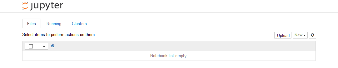
You should now have the running docker instance available on the docker VM, port 8888:

Via the „Upload“ button, upload the Notebook from here: Interactive graphs with Jupyter and R and open it. Execute all steps via „Cell“ -> „Run all“. Now, it should look like:
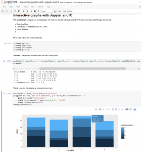
Did you noticed the interactive plot? You can zoom, export as png, have tooltips, … All without anything to programm. Cool, isn’t it?
Ok. Your customer is impressed but does not like the modern html stuff? He wants to print it out and send it away via mail? No problem. Just change the interactive plots to none-interactive ones and export to pdf via „File“ -> „Download as“ -> „PDF via Latex“ (that ’s why the docker file above contains all the stuff like pandoc, latex, …). You will get nearly publication ready report out.